Open-Pit Mine Fugitive Dust Monitoring: Perimeter Station Siting, PM10 Sensors, and AQMS Integration

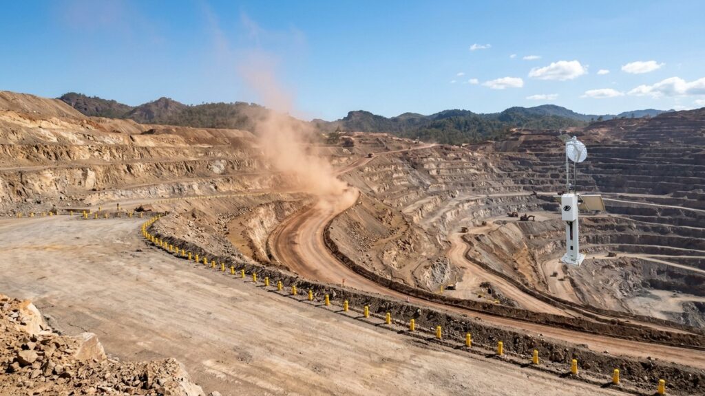
Haul roads pump out 70 to 80 percent of total particulate emissions at an open-pit mine. That makes fugitive dust monitoring a non-negotiable engineering requirement. The figure comes straight from US EPA AP-42 Chapter 11.9 and Chapter 13.2.2. Every dump truck cycle kicks up silt. Every transfer point releases fines. Dust does not wait for a scheduled gravimetric sample.

Manual high-volume air sampling (HVAS) on a six-day cycle captures a snapshot. It cannot warn a shift foreman when PM10 spikes at 2 PM because a water truck broke down. It cannot trigger a mist cannon before the 24-hour average breaches the legal limit. Compliance reporting needs those periodic samples. Operational control needs continuous data.

Indonesian regulations carry teeth. Government Regulation No. 22 of 2021 (PP 22/2021) sets ambient air quality standards with legal force. Minister of Energy and Mineral Resources Decree No. 1827 K/30/MEM/2018 (Kepmen ESDM 1827/2018) adds mining-specific obligations for haul roads, crushers, stockpiles, and transfer points. One exceedance can trigger operational suspension or a community blockade. A monitoring system that misses a dust event costs more in downtime and sanctions than the hardware ever would.

This article covers the engineering of a perimeter dust monitoring network that actually holds up: regulatory thresholds, sensor selection, siting rules, wind-data forensics, and automated water truck dispatch.

Dust Fraction Anatomy: TSP, PM10, and PM2.5 at the Mine Face

Three fractions. Three different behaviors.

TSP (Total Suspended Particulates) covers particles up to roughly 100 µm aerodynamic diameter. Gravity pulls them down fast. Most settle within a few hundred meters of the source. They coat equipment and reduce visibility. Neighbors complain. But TSP rarely travels far enough to trigger a fence-line exceedance on its own.

PM10, the thoracic fraction, tops out at 10 µm. These particles stay airborne for hours. Wind carries them kilometers. They penetrate the upper respiratory tract. At an open-pit mine, haul-road traffic generates the bulk of PM10. AP-42 Chapter 13.2.2 gives the emission factor equation: silt content, vehicle weight, speed, and mitigation efficiency all factor in. Emissions scale linearly with silt loading and vehicle weight, but with the square of vehicle speed. Halving speed cuts emissions by a factor of four. That physics drives the speed-limit component of every TARP.

PM2.5, the respirable fraction, is 2.5 µm and smaller. These linger for days. Sources include diesel exhaust from the fleet and blasting fumes. Coal stockpiles with spontaneous combustion add more. PM2.5 travels the farthest and drives the health complaints from villages downwind.

Aggregate handling and storage piles add another emission stream. AP-42 Chapter 13.2.4 quantifies emissions from material transfer: drop height, wind speed at the drop point, and material moisture content. A dry laterite stockpile in a 5 m/s crosswind releases measurable PM10. A wetted stockpile releases a fraction of that. Same physics at the crusher discharge and the truck dump pocket.

The particle size distribution at a typical laterite nickel mine or thermal coal pit skews coarse at the crusher and stockpile. It skews fine at the haul road when trucks run fast on dry silt. Knowing which fraction dominates where decides sensor placement and technology choice.

Indonesian Ambient Air Quality Thresholds: PP 22/2021 and Kepmen ESDM 1827/2018

Indonesian law sets hard limits. Government Regulation No. 22 of 2021 (PP 22/2021), Annex VII, defines the national ambient air quality standards:

Parameter	24-Hour Average	Annual Average
TSP	230 µg/m³	–
PM10	75 µg/m³	40 µg/m³
PM2.5	55 µg/m³	15 µg/m³

Compliance hinges on the 24-hour running average. Not the peak. Not the one-minute spike. But you need high-resolution data, 1 to 15 minutes, to project whether the daily average will hold. That projection drives operational decisions. A 15-minute average of 120 µg/m³ at 10 AM tells you the daily average is heading for breach. A 15-minute average of 30 µg/m³ at the same hour tells you the day is on track.

The 24-hour average comes from at least 18 valid hourly averages (75 percent data capture). Gaps from power loss or communication failure reduce the valid count. Drop below 18 valid hours and the day is invalid for compliance purposes. Continuous monitoring with local data logging on the datalogger closes this gap, because even if telemetry drops, the hourly average is stored and recovered later.

Minister of Energy and Mineral Resources Decree No. 1827 K/30/MEM/2018 (Kepmen ESDM 1827/2018) adds mining-specific obligations. Annex II and Annex V mandate dust control on haul roads, at crushing facilities, and on stockpiles. Water suppression. Chemical suppressants. Speed limits. Revegetation of exposed areas. The regulation does not prescribe a specific monitoring technology. It requires the outcome: emissions stay within the ambient standards.

The Ministry of Environment and Forestry Regulation No. 14 of 2020 (Permen LHK 14/2020) translates concentrations into the Air Pollution Standard Index (ISPU). Five categories: Good (0-50), Moderate (51-100), Unhealthy (101-200), Very Unhealthy (201-300), Hazardous (>300). Public reporting uses ISPU. Internal control uses raw µg/m³. The conversion is linear piecewise; the breakpoints matter when you automate alert thresholds.

Sensor Metrology: Optical Nephelometer for Operations vs BAM for Legal Compliance

Two instrument classes. Different jobs.

Optical Nephelometer (Light-Scattering Photometer / OPC)

A laser beam crosses a measurement chamber. Particles scatter light. A photodetector converts scatter intensity to mass concentration. Response time: 1 second to 1 minute. Power draw: 5 to 15 watts. Compact enough to run on solar with battery backup at a remote perimeter post.

What it does well: real-time data for TARP triggers, low power, small footprint. It runs continuously without an operator babysitting it.

What it does not do well: the instrument infers mass from optical properties. Particle refractive index and density vary by site. Laterite dust scatters differently than coal dust. A site-specific gravimetric calibration factor (k-factor) must be derived by co-locating the nephelometer with a reference sampler for a representative period. That co-location campaign typically runs 30 days minimum, covering a spread of wind directions and humidity conditions.

Humidity is the killer. At relative humidity above 70-80 percent, hygroscopic particles swell with water vapor. The nephelometer reads the swollen particle as a larger dry particle. False positive. The fix: a smart heated inlet that dries sample air to 50-60 percent RH before it enters the optical chamber. No evaporation of semi-volatile aerosols. Just controlled drying. The heater modulates power to maintain target RH without overshooting. This is not optional in tropical mining environments where dawn RH routinely hits 90 percent.

Optical degradation is the other maintenance item. Silica dust abrades the laser window and photodetector lens. An automated air-purge or wiper system extends service intervals. Without it, monthly cleaning becomes weekly.

Beta Attenuation Monitor (BAM-1020)

Beta radiation from a C-14 source passes through a filter tape collecting particles. Attenuation correlates directly to mass. No optical assumptions. US EPA designates it a Federal Equivalent Method (FEM). It is the legal-reference standard for 24-hour compliance reporting.

Trade-offs: one-hour measurement cycle typical. Power consumption in the hundreds of watts, so it needs grid or generator. High capital cost. Consumable filter tape. Maintenance-heavy. Not practical for a string of solar-powered perimeter nodes.

The BAM heated inlet is standard equipment. It maintains sample RH below 50 percent by design. The tape advance mechanism and beta detector require quarterly calibration checks. The pump and flow controller need annual servicing. Budget for both.

Hybrid Strategy

Deploy nephelometers across the operational perimeter for real-time control. Co-locate one BAM at the most sensitive receptor (usually the village boundary downwind) for legal defensibility. Cross-calibrate the optical fleet against the BAM quarterly. This gives you both operational speed and audit-grade data.

For deeper comparison, see the technical breakdown of BAM vs OPC sensor selection. The humidity compensation mechanism is detailed in PM2.5 sensor humidity bias mitigation.

Perimeter Station Siting: AS/NZS 3580.1.1 Criteria and Upwind-Downwind Architecture

Bad siting produces bad data. A sensor behind a berm reads turbulence, not ambient air. A sensor on the pit rim reads flyrock dust, not fence-line exposure. International standards exist for a reason.

AS/NZS 3580.1.1:2016 and US EPA 40 CFR Part 58 Appendix E align on the fundamentals:

• Inlet height: 2.0 to 7.0 meters above ground for neighborhood/micro scale. This avoids ground-level dust resuspension and captures the breathing zone.
• Obstruction clearance: horizontal distance at least twice the height of any nearby obstacle (building, tree, stockpile, berm). A 5-meter tree demands 10 meters of clearance.
• Unrestricted airflow arc: minimum 270 degrees. On an open mast at the concession boundary, 360 degrees is achievable.
• Stable ground: the station sits on the legal concession boundary (fence-line / IUP boundary), geotechnically stable, outside the blast flyrock zone. Not on the active pit crest.

The inlet height range is not arbitrary. Below 2 meters, the sampler ingests mechanically resuspended dust from vehicle wakes and wind erosion of bare soil. Above 7 meters, the sampler may miss the plume core from ground-level sources. The 2-7 meter window captures the well-mixed layer for neighborhood-scale monitoring.

Upwind-Downwind Architecture

Minimum viable network: one upwind station, two to four downwind stations.

The upwind station captures background: regional haze, bushfire smoke, highway traffic, village cooking fires. Downwind stations sit where the wind carries mine emissions toward sensitive receptors like settlements, plantations, or water intakes.

Indonesia reverses wind direction between the Northwest Monsoon (Muson Barat) and Southeast Monsoon (Muson Timur). A station that is upwind in July becomes downwind in January. Historical wind rose analysis, at least five years of data, determines the seasonal flip points. The network design has to account for both regimes. Some concessions install dual-role stations that work as upwind in one season and downwind in the other, provided the siting criteria hold for both roles.

Concession size matters. A 500-hectare pit may need only three perimeter stations. A 5,000-hectare concession with multiple active pits and a dispersed haul network may need eight to twelve. The rule of thumb: every active haul road segment and every active dump face needs a downwind station within the dominant transport sector for the current season.

Mass Balance Formula

The net mine contribution at the boundary is arithmetic:

C_net = C_downwind – C_upwind

Same time interval. Same averaging period. If upwind reads 60 µg/m³ PM10 and downwind reads 95 µg/m³, the mine adds 35 µg/m³. If upwind reads 80 µg/m³ and downwind reads 85 µg/m³, the mine adds only 5 µg/m³, meaning the exceedance is imported, not yours.

This calculation wins regulatory disputes more often than anything else in the toolbox. It requires synchronized timestamps, matched averaging periods, and validated instruments on both ends. Time synchronization across the network must be better than 1 minute. NTP over cellular or GPS-disciplined clocks handle this.

AQMS and Weather Station Integration: Wind Rose, Bivariate Polar Plots, and Source Apportionment

A particulate sensor without a co-located weather station is a blind sensor. You get concentration. You do not get origin.

Ultrasonic Anemometer

Mechanical cup-and-vane anemometers seize up in silica dust. Bearings fail. Vanes stick. Ultrasonic anemometers have no moving parts. They measure wind speed and direction by time-of-flight of sound pulses. Zero maintenance in dusty air. They also output sonic temperature, a useful cross-check.

See the ultrasonic vs cup-and-vane comparison for the full trade-off analysis.

Wind Rose

A wind rose plots frequency of wind direction by speed class. Seasonal roses for the concession reveal the dominant transport pathways. In Sumatra coal basins, the northwest monsoon pushes dust toward the coast. In Kalimantan, the southeast monsoon drives it inland. The rose tells you where to put the downwind stations.

The rose also reveals calms. Hours with wind speed below 0.5 m/s produce stagnation. PM10 accumulates locally. A TARP that ignores calms will miss the worst buildup events. The polar plot handles this; the rose does not.

Bivariate Polar Plot

This is the forensic tool. Concentration mapped as a function of wind direction (0–360°) and wind speed (m/s). The method (Grange, Lewis & Carslaw, 2016) separates sources by their wind-speed signature:

• Local ground-level sources (haul roads, stockpiles): high concentrations at low wind speeds (1-3 m/s), narrow directional sector.
• Elevated or distant sources (regional haze, stack emissions): high concentrations at higher wind speeds (5-10 m/s), broader sectors.
• Vehicle exhaust (diesel PM2.5): appears at very low wind speeds, often centered on the access road alignment.

Overlay the polar plot on the site plan. The hotspot aligns with the haul road? That is your source. The hotspot aligns with the highway outside the concession? That is not your source.

This analysis turns monitoring data into legal evidence. It also guides mitigation: if the polar plot fingers the crusher transfer point at low wind speed, a mist cannon there solves more than watering the entire haul road.

The polar plot requires simultaneous high-resolution PM10 and wind data. A 15-minute average is the practical minimum. Hourly averages smear the signal. The edge datalogger computes the plot incrementally and pushes the updated image to the dashboard every cycle.

Automated Dust Control via TARP: From Sensor Signal to Water Truck Dispatch

Data without action is noise. A Trigger Action Response Plan (TARP) converts concentration thresholds into prescribed operational responses. The goal: intervene before the 24-hour average breaches 75 µg/m³ PM10.

TARP Level Definitions

The following table defines a four-level TARP based on 15-minute and 1-hour rolling averages of PM10. Thresholds are illustrative; each site calibrates to its background and receptor sensitivity.

Level	Label	15-min Rolling Avg PM10 (µg/m³)	1-hr Rolling Avg PM10 (µg/m³)	Mandatory Actions
1	Green – Normal	< 50	< 40	Standard operations. Routine watering schedule. Continuous monitoring.
2	Yellow – Alert	50-100	40-75	Radio notification to shift foreman. Water truck fleet staged at critical haul-road segments. Wind direction verified. Dust suppressant stock checked.
3	Orange – High	100-150	75-120	Automatic dispatch of water trucks to active haul segments. Mist cannons activated at crusher and transfer points. Chemical suppressant applied to high-silt sections. Haul truck speed reduced from 40 km/h to 25 km/h on affected segments.
4	Red – Critical	> 150	> 120	Mandatory speed limit 20 km/h on all haul roads. Suspend dumping at exposed windward benches. Full fleet water truck deployment. Incident report to KTT and environmental manager. Prepare regulatory notification if 24-hr projection exceeds limit.

The thresholds above use 15-minute and 1-hour rolling averages. Some jurisdictions prefer a 1-hour and 24-hour pair. The principle holds: shorter averaging periods trigger earlier; longer periods confirm trend. The TARP must specify which average governs each level transition.

Sensor Comparison Matrix

Criterion	Nephelometer (OPC)	BAM-1020 (FEM)
Measurement principle	Laser light scattering	Beta attenuation
Time resolution	1 sec – 1 min	1 hour typical
Power consumption	5-15 W (solar viable)	200-400 W (grid/gen)
Capital cost	Low	High
Operating cost	Low (no consumables)	Medium (filter tape, pump)
Legal standing	Indicative / operational	Federal Equivalent Method
Humidity sensitivity	High (needs heated inlet)	Low (heated inlet standard)
Calibration	Site-specific k-factor vs gravimetric	Factory calibrated, periodic audit
Best fit	Perimeter network, TARP trigger	Compliance reference station

Telemetry and Edge Computing

The TARP logic runs at the edge. A ruggedized datalogger, such as the GEOVOS unit, computes rolling averages, evaluates wind vectors, and fires relay outputs or MQTT messages to the mine’s Fleet Management System (FMS) without cloud latency. Dual-path telemetry (cellular primary, satellite backup) keeps the loop closed in remote concessions.

Fortuna Argatech integrates the AQMS particulate station, the ultrasonic AWS, the smart heated inlet, and the GEOVOS datalogger into a single solar-powered enclosure rated IP66. The edge processor handles the TARP state machine locally. The dashboard shows real-time PM10, wind rose, polar plot, and TARP level per station. Water truck dispatch receives the alert on the same screen they use for haul-cycle management.

This is not a concept diagram. It is the architecture running at remote mine sites where grid power does not exist and a missed dust event means a regulatory sanction or a community road blockade.

The edge processor also logs every TARP state change with timestamp, concentration, wind vector, and action triggered. This log is the audit trail. When the regulator asks why the water truck was not dispatched at 14:32 on June 12, the log answers. A handwritten logbook does not.

Implementation Path

Start with a desktop study. Pull five years of hourly wind data from the nearest BMKG station or on-site met mast. Generate seasonal wind roses. Identify candidate upwind and downwind positions per AS/NZS 3580.1.1. Then walk the boundary yourself. Verify obstruction clearance, geotechnical stability, and check that the station will still be there after the next blast.

Select instruments. Nephelometers with heated inlets for the perimeter array. One BAM at whichever receptor faces the most community exposure. Ultrasonic anemometers co-located at every particulate node. Size solar arrays for 5-day autonomy at worst-case monsoon insolation. Include battery capacity for 72 hours of continuous operation without sun.

Commission with a 30-day co-location campaign against a gravimetric reference. Derive k-factors. Validate the TARP thresholds against observed background. Train the shift foremen on the dashboard and make them use it during handover. Document the SOP. The SOP must cover: sensor cleaning schedule, heated inlet verification, flow rate checks, time synchronization check, TARP threshold adjustment procedure, and escalation matrix for communication failures.

Calibrate quarterly. Audit annually. Replace filter tape on the BAM per manufacturer schedule. Clean nephelometer optics on the preventive maintenance cycle. The system survives because the maintenance plan is built in, not bolted on after commissioning.

Perimeter dust monitoring at an open-pit mine is not something you buy and forget. The hardware enables control. Good siting validates the data. Wind forensics defend you in a dispute. The TARP closes the loop between sensor and water truck. Miss any piece and the investment underperforms.

Budget for the full lifecycle. Capital covers hardware, mast structures, solar arrays, and commissioning. Operating expense covers quarterly calibration, annual audit, consumable replacement (BAM filter tape, desiccant), and cellular or satellite data plans. A typical three-station perimeter network with one BAM reference station runs 15-20 percent of capital per year in OPEX. Factor this into the project economics from day one.

For the canonical AQMS platform that supports this architecture, see the Air Quality Monitoring System product page. The matching industrial weather station provides the ultrasonic wind data. ISPU conversion from sensor data is covered in calculating ISPU from AQMS sensor data. For mining operations managing multiple environmental vectors, environmental noise monitoring sensors for industrial compliance addresses the parallel noise obligation.