Why Safety Gas Detectors Fail at Odor Monitoring: Choosing ppb-Level H2S Sensors and Fenceline E-Noses

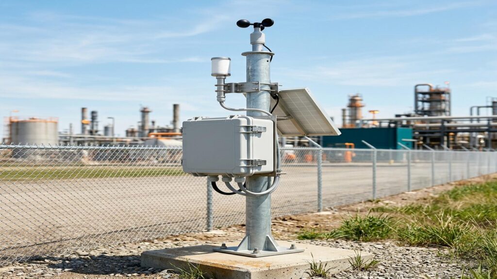
Your plant’s fixed H2S safety detectors read 0.0 ppm. The control room sees green lights across the board. Meanwhile, residents three kilometers downwind are filing complaints about rotten-egg smell, threatening regulatory action, and organizing protests. This scenario plays out at wastewater plants, palm oil mills, landfills, and chemical parks across Indonesia every week. The root cause isn’t instrument failure. It’s a metrology mismatch. Safety detectors operate on the ppm scale. Odor regulation and human noses operate on the ppb scale. This article breaks down why that gap matters, which sensor technologies actually close it, and how to build a fenceline monitoring system that holds up under scrutiny.

The Metrology Gap: Why ppm-Scale Safety Detectors Are Blind to Odor

Human olfactory threshold for hydrogen sulfide sits between 0.5 and 8 parts per billion. The World Health Organization documents this range in its Air Quality Guidelines for Europe. At 15–20 ppb, communities smell it clearly and complain. Indonesia’s ambient odor standard under Kepmen LH No. 50/1996 caps H2S at 0.02 ppm (that’s 20 ppb). Yet the occupational health and safety limit under Permenaker No. 5/2018 sets the 8-hour time-weighted average at 1 ppm. That’s a 50-fold difference between the worker safety threshold and the environmental odor threshold.

Standard industrial safety detectors (the fixed heads you mount near reactors, lift stations, and confined spaces) typically range 0–50 ppm with 0.1 ppm resolution. At 20 ppb, they display 0.0. At 100 ppb, they still display 0.0. The instrument isn’t broken. It’s simply operating two orders of magnitude above the concentration range that triggers odor complaints and regulatory violations.

This isn’t theoretical. For example, when a wastewater treatment plant’s aeration basin turns anaerobic at 3 AM, H2S can spike to an illustrative 30–50 ppb at the fenceline. Neighbors wake up. The plant’s safety dashboard shows zeros. By morning, the environmental agency has a formal complaint. The plant manager learns the hard way that “zero on the safety panel” does not mean “zero odor impact.”

Bottom line: if odor compliance or community relations are part of your brief, ppm-scale safety detectors won’t cut it. You need trace-level sensors with detection limits below 2 ppb and single-digit ppb resolution.

Key Industrial Odorants and Indonesia’s Odor Emission Standards

Kepmen LH No. 50/1996 regulates five specific odorants with individual ambient limits:

Odorant	Limit (ppm)	Limit (ppb)
Ammonia (NH3)	2.0	2,000
Methyl mercaptan (CH3SH)	0.002	2
Hydrogen sulfide (H2S)	0.02	20
Methyl sulfide (CH3SCH3)	0.01	10
Styrene (C8H8)	0.1	100

Methyl mercaptan carries the tightest limit at 2 ppb. Any credible continuous monitor needs sub-ppb detection capability to cover it. Ammonia and H2S dominate at wastewater treatment plants, landfills, and palm oil mill effluent (POME) ponds. Styrene appears in petrochemical and plastics facilities. Methyl sulfide shows up in pulp and paper, and certain chemical synthesis operations.

PP No. 22/2021 Articles 207–208 classifies odor alongside noise and vibration as a “nuisance standard” (baku mutu gangguan) that must be controlled under environmental permits. Kepmen LH 50/1996 mandates quarterly monitoring reports to the environmental agency. Miss a report, exceed a limit, or ignore a complaint, and you’re looking at enforcement pathways that can escalate to operational suspension.

The regulatory framework is clear: you must demonstrate compliance at the fenceline, not at the stack. Stack monitoring tells you what you emit. Fenceline monitoring tells you what the neighbor breathes. They are not the same, especially under nocturnal temperature inversion when emissions hug the ground and travel kilometers.

Technology Comparison: ppb Electrochemical Cells vs E-Nose (IOMS) vs Optical Spectrometry

Three technology families compete for fenceline odor monitoring. Each works differently, gets treated differently by regulators, and costs differently.

ppb-Level Electrochemical Sensors (4-Electrode Architecture)

Sensors like the Alphasense H2S-B4 use a four-electrode design: working electrode (WE), counter electrode (CE), reference electrode (RE), and an auxiliary electrode (AE). The AE tracks the zero-current baseline in real time, compensating for thermal drift that plagues two- and three-electrode cells. Limit of detection reaches below 2 ppb. Measurement range spans 0–2 ppm, wide enough for odor monitoring but narrow enough to keep ppb resolution.

These sensors output a linear current proportional to H2S concentration. They’re specific to the target gas, though cross-sensitivity to other sulfur compounds exists and must be characterized. In tropical field deployments, electrochemical H2S cells typically last 18–24 months before electrolyte depletion or electrode fouling requires replacement.

The upside: you get a direct concentration readout in ppb, traceable to gas calibration standards. The downside: it’s single-gas measurement. If your odor profile includes methyl mercaptan, ammonia, and styrene simultaneously, you need multiple probes or a different approach.

Instrumental Odour Monitoring Systems (IOMS / E-Nose)

E-Nose systems don’t measure individual gas concentrations. They measure “odour concentration” in European Odour Units per cubic meter (ou_E/m³) per EN 13725. A multi-sensor array, typically combining metal oxide semiconductor (MOS), electrochemical, and sometimes photoionization detectors, generates a response pattern. Chemometric algorithms (pattern recognition, partial least squares regression, neural networks) map that pattern to an odour concentration estimate calibrated against dynamic olfactometry panels.

CEN/TS 17433 and VDI 3518 define verification protocols for IOMS: linearity, repeatability, detection limit, drift, and field validation against EN 13725 olfactometry. An IOMS that passes CEN/TS 17433 verification serves as a continuous screening tool alongside periodic human-panel olfactometry, not a replacement for it.

What you gain: one instrument captures the combined odor fingerprint of complex mixtures. What you lose: the ou_E/m³ output is an estimate, not a direct chemical measurement. Regulatory acceptance in Indonesia still references Kepmen LH 50/1996’s single-compound limits. IOMS data supports early warning and trend tracking; it does not replace laboratory reference methods for legal compliance reporting.

UV-Fluorescence Optical Analyzers

UV-fluorescence (UVF) analyzers for H2S and SO2 offer the highest stability and lowest drift of any continuous method. No consumable electrolyte, no electrode aging, no membrane replacement. Detection limits reach sub-ppb. Selectivity is tight. UVF responds almost exclusively to the target molecule.

On the plus side: multi-year stability with almost no maintenance. On the minus side: capital cost runs 3–5× higher than electrochemical probes. For a multi-point fenceline deployment, UVF at every station is rarely budget-justifiable. Most operators reserve UVF for a single reference station and deploy electrochemical sensors at perimeter points.

---

Comparison Matrix: Fenceline Odor Monitoring Technologies

Parameter	Safety Detector (ppm)	ppb Electrochemical	E-Nose / IOMS	UV-Fluorescence
Measurement unit	ppm	ppb (µg/m³)	ou_E/m³	ppb (µg/m³)
Limit of detection	~100 ppb	<2 ppb	~5–10 ou_E/m³	<1 ppb
Target specificity	Single gas (H2S)	Single gas (H2S, NH3, etc.)	Multi-odorant fingerprint	Single gas (H2S, SO2)
Regulatory alignment (Kepmen LH 50/1996)	No — wrong scale	Yes — direct ppb readout	Indirect — ou_E/m³ surrogate	Yes — direct ppb readout
Thermal drift compensation	None	4-electrode AE correction	Algorithm-dependent	Minimal (optical stability)
Humidity transient immunity	Poor	Moderate (with conditioning)	Variable (MOS sensitive)	High
Sensor lifespan (tropical)	2–3 years	18–24 months	12–24 months (MOS array)	5+ years (optical bench)
Typical CAPEX per point	Low	Medium	High	Very High
OPEX (consumables)	Low	Electrolyte/cell replacement	Sensor array replacement	Minimal (lamp, filters)

---

Choosing the Right Approach

The right combination depends on your emission profile and regulatory exposure. For a single dominant odorant like H2S or NH3, ppb electrochemical probes at 3–5 perimeter points plus one upwind background station cover Kepmen LH 50/1996 compliance at the lowest cost tier. For complex odor mixtures with high complaint risk, adding an E-Nose (IOMS) at the primary downwind receptor point captures the total odor fingerprint while electrochemical probes handle legally referenceable single-compound data; expect E-Nose systems to cost 3–5× more than single-gas electrochemical probes. For maximum legal defensibility, a UV-fluorescence reference analyzer at the main fenceline station field-validates the electrochemical network, though at the highest capital outlay. Regardless of configuration, plan for quarterly calibration verification per Kepmen LH 50/1996 and sensor cell replacement every 18–24 months.

Tropical Field Challenges: Humidity Transients, Drift, and Sensor Poisoning

Indonesia’s climate breaks instruments designed for temperate zones. Three failure modes kill field deployments.

RH shock transients. A sudden downpour or morning fog can swing relative humidity from 60% to 95% in minutes. In electrochemical cells, this step change induces a transient current spike that the instrument interprets as a gas concentration jump. Without mitigation, you get false alarms every time a storm passes. The four-electrode architecture’s auxiliary electrode corrects baseline drift from temperature, but humidity transients require additional handling: hydrophobic ePTFE membrane filters on the sample inlet, mild heating (2–3°C above ambient) to prevent condensation, and firmware algorithms that flag and suppress RH-induced transients.

Thermal baseline drift. Daily temperature swings of 10–15°C in exposed enclosures shift the zero current of two- and three-electrode cells by tens of ppb equivalent. The auxiliary electrode in 4-electrode designs tracks this in real time. For single-gas ppb probes, you can’t skip this compensation. Without it, your midnight baseline reads 15 ppb and your noon baseline reads 5 ppb. Not because H2S changed, but because the sensor electronics drifted.

Sulfur poisoning of MOS sensors. Metal oxide semiconductor sensors, common in E-Nose arrays, degrade irreversibly under sustained high-concentration sulfur exposure. At a palm oil mill where H2S routinely hits 5–10 ppm near the anaerobic ponds, MOS elements can lose sensitivity or shift baseline within months. Electrochemical cells tolerate high concentrations better but still consume electrolyte faster. Plan for 18–24 month cell replacement cycles in aggressive environments. Budget for it.

Sample conditioning is not optional. Every outdoor trace-gas probe needs: a heated sample line or inlet heater (2–3°C above dew point), hydrophobic membrane filter (ePTFE, 0.2–0.45 µm), particulate pre-filter, and a weatherproof enclosure with active ventilation. Skip any of these and your data quality degrades within weeks.

Integrating Weather Stations for Odor Dispersion Tracking and Legal Defense

Gas concentration data without wind vector is legally indefensible. If a complaint arrives at 6 AM alleging odor from your plant, and your fenceline sensor recorded 25 ppb H2S at 5:45 AM, you need to prove whether that plume came from your facility or from the landfill two kilometers upwind. Without synchronized wind direction and speed at the same timestamp, you have a number, not a defense.

Ultrasonic 2D anemometers are the standard for fenceline work. No moving parts means no mechanical inertia. They detect wind direction and speed down to near-zero thresholds. That matters because odor accumulates during calm, stable nighttime conditions when cup anemometers stall. Mount the anemometer on a 3–10 meter mast per WMO siting guidelines, clear of building turbulence zones.

With synchronized gas and wind data, you build two analytical products:

Wind rose + polar plot. Plot H2S concentration as a function of wind direction. If high concentrations cluster when wind blows from your process area toward the receptor, the evidence points to your plant. If they cluster when wind blows from a neighboring facility, you have exculpatory data. Polar plots visualize this instantly for regulators and community meetings.

Back-trajectory dispersion analysis. For deeper investigation, feed the fenceline time series into a Gaussian plume model (AERMOD, CALPUFF) with local terrain and building downwash. This reconstructs the probable source location. It’s not a substitute for stack monitoring. It’s a complement that answers “where did this specific plume originate?”

Nocturnal thermal inversion is the meteorological amplifier. On clear, calm nights, the ground cools faster than the air above, creating a stable layer that traps pollutants near the surface. H2S emitted at 10 PM can accumulate to 5–10× daytime concentrations at the fenceline by 3 AM. Your monitoring system must capture this diurnal pattern. A single daytime grab sample misses it entirely.

Argatech Fenceline Monitoring Architecture: From Sensor to Telemetry Dashboard

Fortuna Argatech builds integrated fenceline monitoring systems, not loose sensors. The architecture centers on the AQMS platform configured with trace-level gas probes, synchronized with an Automatic Weather Station (AWS), feeding an industrial data logger, and transmitting via cellular or satellite telemetry to a centralized dashboard.

Sensor layer. The AQMS accepts ppb-range electrochemical probes for H2S, NH3, and other odorants via Modbus RS485. Each probe includes integrated sample conditioning: heated inlet, hydrophobic membrane, particulate filter. For multi-odorant sites, an E-Nose module (IOMS) can be added to the same data logger bus, outputting ou_E/m³ alongside the single-gas ppb channels.

Meteorological layer. The Argatech AWS mounts an ultrasonic 2D anemometer, temperature, humidity, barometric pressure, and optional solar radiation sensors. All meteorological data shares the same Modbus RS485 backbone and timestamp base as the gas data. No clock drift between instruments. No manual alignment in post-processing.

Data logger and telemetry. An industrial-grade data logger (DIN-rail, wide-temperature, watchdog-supervised) polls all Modbus devices at configurable intervals, typically 10–60 seconds for gas, 1 second for wind. It computes rolling averages (1-minute, 5-minute, 15-minute, 1-hour), applies calibration coefficients, flags sensor faults, and buffers data during communication outages. Transmission uses 4G/LTE with fallback to LoRa or satellite for remote sites. End-to-end encryption, MQTT or HTTPS to the cloud platform.

Dashboard and alarm. The telemetry dashboard displays real-time gas concentrations, wind vectors, polar plots, and wind roses. Tiered alarm logic: Level 1 (early warning) at 50% of odor threshold, triggering internal notification via WhatsApp and email. Level 2 (action threshold) at 100%, triggering operator response protocol. Level 3 (exceedance) at regulatory limit, auto-generating an incident report with timestamped gas and wind data for regulatory submission. Historical query, CSV export, and API access for integration with plant SCADA or corporate ESG reporting.

Why integration matters. A standalone ppb sensor tells you “H2S is 18 ppb.” An integrated system tells you “H2S is 18 ppb, wind is 1.2 m/s from 225°, polar plot shows this plume originates from the anaerobic lagoon, alarm Level 1 active, operator notified.” That’s the difference between a data point and a decision-support tool.

Internal References

• Environmental noise monitoring as complementary nuisance parameter: Environmental Noise Monitoring Sensors
• Electrochemical sensor cross-sensitivity deep dive: Electrochemical Gas Sensor AQMS Cross-Sensitivity
• VOC sensor technology comparison (PID vs NDIR vs MOS): Gas Sensor VOC AQMS PID vs NDIR vs MOS
• Ultrasonic anemometer selection for fenceline: Ultrasonic vs Cup and Vane Anemometer
• Humidity bias mitigation for outdoor sensors: Humidity Bias PM2.5 Sensor

---

External Authoritative Sources

1. WHO Air Quality Guidelines for Europe, Chapter 5.6 Hydrogen Sulfide (2000) — olfactory threshold 0.5–8 ppb
2. Kepmen LH No. 50/1996 — Indonesian ambient odor standards for 5 odorants
3. Permenaker No. 5/2018 — occupational H2S exposure limits (1 ppm TWA)
4. EN 13725:2022 — dynamic olfactometry and European Odour Unit definition
5. CEN/TS 17433:2021 & VDI 3518 — IOMS/E-Nose verification standards
6. Alphasense Application Note AAN 114 & H2S-B4 Datasheet — 4-electrode ppb sensor specifications
7. PP No. 22/2021 Articles 207–208 — odor as environmental nuisance standard
8. US EPA Fenceline Monitoring Technologies — dispersion correlation methodology
9. Ellona WT1 Fenceline Monitoring System — integrated gas + ultrasonic anemometer reference architecture

---

Fortuna Argatech designs and integrates custom fenceline odor monitoring systems for wastewater treatment, palm oil, petrochemical, landfill, and heavy industrial facilities across Indonesia. Contact our engineering team to discuss your site-specific requirements.