Turbidity vs TSS: Which Measurement Fits Your Water System?

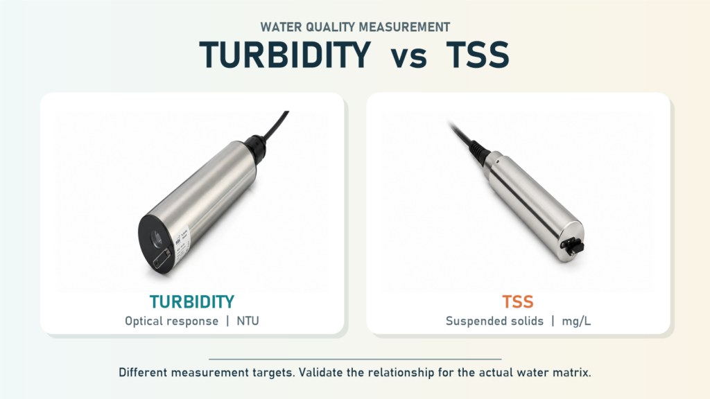
Turbidity vs TSS is a comparison between two measurements that respond to particles in water but do not measure the same property. Turbidity describes an optical response to light, while Total Suspended Solids (TSS) expresses the mass concentration of suspended material in a volume of water.

That distinction affects the units, reference method, maintenance plan, and decisions the data can support. Turbidity is valuable for rapid process trends, but its reading should not be relabeled as TSS unless a relationship has been established for the actual water matrix and operating range.

Fortuna Argatech maintains official pages for a Turbidity Sensor and an online TSS Sensor. Both support online monitoring and RS485 Modbus integration. A shared communication interface, however, does not make their measurement meaning interchangeable.

Turbidity vs TSS starts with the measurement target

The USGS overview of turbidity describes it as relative clarity measured through the light scattered by material in water. Under a nephelometric method, results are commonly reported in Nephelometric Turbidity Units (NTU). A higher optical response under that method produces a higher turbidity value.

TSS takes a different route. In a gravimetric laboratory context, a known sample volume is processed, the retained solids are dried, and their mass is used to calculate a concentration in milligrams per liter (mg/L). A USGS comparison of suspended-solids analytical data also shows why sample handling and analytical procedure matter; the parameter name alone does not describe every source of measurement difference.

Area	Turbidity	TSS
Main question	How strongly does the water scatter or absorb light?	What is the mass concentration of suspended solids in the sample?
Common unit	NTU for a nephelometric method	mg/L
Reference approach	Optical response against turbidity standards	Sample processing and gravimetric mass determination
Operational strength	Fast, continuous trends and early detection of change	Direct connection to a mass-concentration result required in many water-quality evaluations
Important limitation	Affected by particle properties, water color, sensor optics, bubbles, and fouling	Affected by sample representativeness, subsampling, filtration, drying, and weighing procedures

An online TSS probe can also use an optical principle while displaying mg/L. It does not dry and weigh solids inside the sensor. Instead, its optical signal is converted to an estimated concentration through calibration. The project therefore needs to understand the calibration reference, the water matrix, and the comparison evidence behind the displayed value.

Why NTU does not have one universal mg/L conversion

Water samples containing the same mass of solids can scatter light differently. Fine and coarse particles do not create the same optical response. Shape, color, composition, microorganisms, and the sensor’s light source and detector geometry can also change the result.

USGS Techniques and Methods 3-C4 explicitly treats turbidity as an optical index rather than a direct particle-mass measurement. Its workflow combines turbidity readings with measured suspended-sediment samples to develop a site-specific regression model. Continued reference samples are needed because sediment sources and characteristics can change.

A formula developed at a wastewater inlet may therefore fail at the outlet, in a river, at a mine-water point, or at another facility. Even at one location, a new raw material, seasonal runoff, coagulant adjustment, biological growth, or change in the dominant particle type can shift the relationship.

A strong correlation during one campaign is not permission to stop reference testing permanently. The model needs a defined scope, an operating range, rules for values outside that range, and a verification schedule based on the data objective and risk.

Select the parameter from the decision it must support

Do not begin with which sensor sounds more advanced. Begin with the action that follows the number on the dashboard.

Need	More relevant starting point	Verification note
Detect a clarity change, filter disturbance, or sudden particle event quickly	Continuous turbidity	Establish the process baseline, installation location, alarm logic, and fouling response
Determine a solids mass concentration using a required method	TSS with the appropriate reference procedure	Confirm the method, sampling procedure, laboratory, and reporting requirement
Estimate TSS continuously for process control	Online TSS sensor or a turbidity-based model	Use paired samples and demonstrate performance in the actual matrix and operating range
Combine rapid trend detection with periodic reference results	Optical monitoring plus laboratory samples	Use reference results to check bias, drift, and changes in the relationship

If a permit, contract, or internal procedure explicitly requires TSS, do not substitute turbidity merely because the two charts look similar. The team must confirm the applicable parameter and method. Conversely, if the main need is a process response within minutes, laboratory sampling alone can leave a long information gap.

Verify the sensor before using it as a TSS estimator

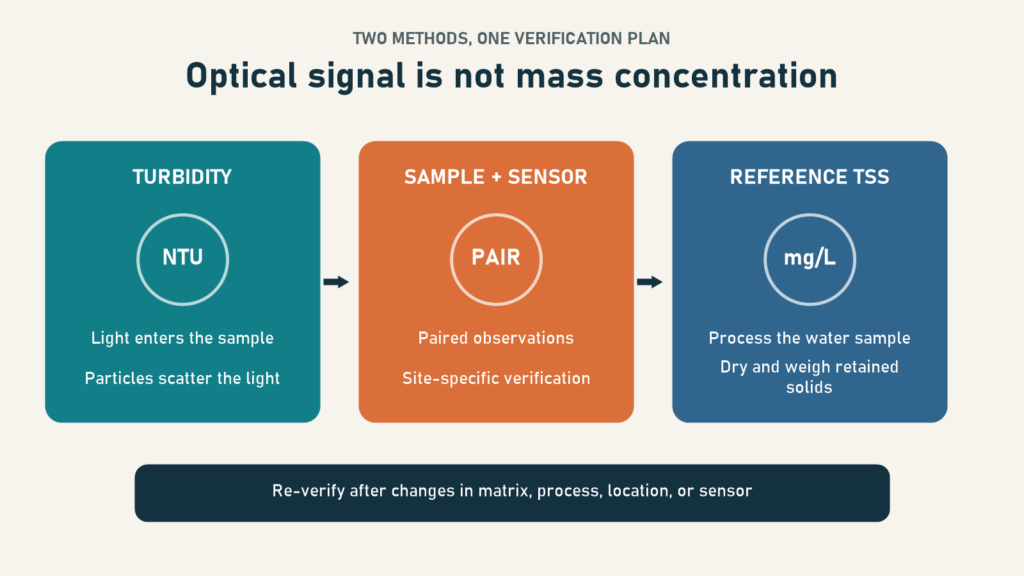
1. Define the objective and reference method

State whether the data supports a process alarm, treatment optimization, reporting, event investigation, or several of these tasks. Identify the reference method and unit that will be used to judge performance.

2. Choose a representative measurement point

The sensor and sample location should represent the same water. Review mixing, settling, bubbles, changing water level, access for cleaning, and whether the probe may sit in a dead zone that differs from the main flow.

3. Collect paired data across relevant conditions

Record the sensor reading at a time aligned with reference sampling. The data set should cover the intended operating range, not only stable normal conditions. Document process changes, rainfall, chemical dosing, cleaning, and sensor disturbances.

4. Evaluate the relationship and its errors

Do not judge the model from a correlation coefficient alone. Review bias, residuals, calibration range, extreme values, and whether different operating conditions form different relationships. Qualified personnel should select the model and acceptance criteria based on the analytical method and operational objective.

5. Test with data not used to build the model

Verification data reveals whether the relationship works outside the original calibration set. If it does not meet the need, correct the location, sampling procedure, configuration, or model before expanding the deployment.

6. Define re-verification triggers

Review the relationship after changes in the process, water source, solids type, chemical treatment, probe location, or sensor components. Keep the model version, validity period, and change record so historical dashboard values remain explainable.

Maintenance determines whether the trend remains credible

An optical window covered by biofilm, sludge, or bubbles can change the signal even when the water has not changed. An automatic cleaning mechanism helps, but it does not remove the need for inspection.

The USGS continuous water-quality monitor guidance separates fouling effects from calibration drift by documenting readings before cleaning, after cleaning, and during standard checks. It does not support one universal service interval; site conditions, season, sensor type, and data-quality objectives affect the schedule.

An operating plan should identify who cleans the probe, how inspections are recorded, when reference samples are collected, and what action follows an implausible or out-of-range value. The related Argatech guide to environmental sensor calibration provides broader maintenance context.

Design the monitoring system, not only the probe

A sensor value becomes useful when its parameter identity, unit, timestamp, quality status, and calibration history remain intact through the dashboard. A data logger, PLC, or SCADA system should map the registers correctly and distinguish raw readings, corrected readings, and model-based estimates.

A technical discussion with Fortuna Argatech can start with the required parameter, water matrix, reference method, maintenance access, RS485 Modbus connection, and the path from the field sensor to the dashboard. This keeps the selection focused on operational decisions rather than on a specification sheet alone.

For a broader parameter overview, read four wastewater quality parameters to monitor. If your project needs to separate turbidity, laboratory TSS, and online TSS estimation, contact Fortuna Argatech to discuss the matrix, integration, and verification plan.

Sources

• U.S. Geological Survey. Turbidity and Water. https://www.usgs.gov/special-topics/water-science-school/science/turbidity-and-water
• U.S. Environmental Protection Agency. Method 180.1: Determination of Turbidity by Nephelometry, Revision 2.0. https://www.epa.gov/sites/default/files/2015-08/documents/method_180-1_1993.pdf
• U.S. Geological Survey. Guidelines and Procedures for Computing Time-Series Suspended-Sediment Concentrations and Loads from In-Stream Turbidity-Sensor and Streamflow Data. https://pubs.usgs.gov/tm/tm3c4/
• U.S. Geological Survey. Comparability of Suspended-Sediment Concentration and Total Suspended Solids Data. https://pubs.usgs.gov/wri/wri004191/
• U.S. Geological Survey. Guidelines and Standard Procedures for Continuous Water-Quality Monitors. https://pubs.usgs.gov/tm/2006/tm1D3/