Area-Velocity Acoustic Doppler Flow Sensors: Measuring Discharge in Non-Standard Open Channels and Partially Filled Pipes

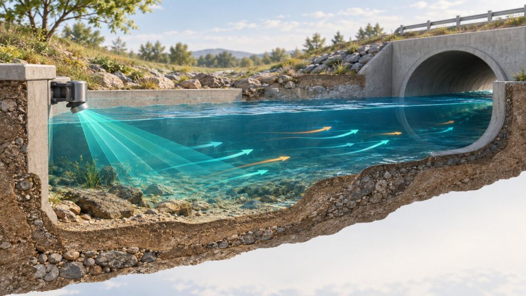
The SPARING framework (Permen LHK No. P.80/2019) requires continuous wastewater discharge monitoring. The mandate sets a strict accuracy tolerance of $\pm 10%$. That number matters. Flow data directly drives the daily pollution load calculations reported to regulators. Miss the flow measurement, and your entire environmental compliance record collapses.

Most wastewater treatment plant (WWTP) engineers default to primary hydraulic structures. They build Parshall flumes or weirs. In a textbook, that works perfectly. In the field, reality hits hard. Aging industrial outfalls often feature flat hydraulic gradients. Channels have irregular cross-sections. Some rely on underground circular concrete culverts flowing partially full. You simply cannot squeeze a standard flume into these restrictive spaces.

Enter area-velocity flow sensors. Powered by acoustic Doppler technology, these instruments provide a direct volumetric measurement solution. You get reliable flow data without pouring concrete for an artificial calibration structure.

Why Flumes and Weirs Fail in Non-Standard Channels and Flat Effluents

Primary hydraulic structures demand vertical head loss. A Parshall flume forces a hydraulic transition. It chokes the subcritical flow into a critical state (Froude number, $Fr = 1$) at the throat. We need that critical flow. It establishes the deterministic mathematical relationship between water head and volumetric discharge.

Now try dropping a flume into a flat gradient industrial effluent channel. You create a massive bottleneck. The structure generates upstream backwater effects. Wastewater pools backward. It climbs up the pipes toward the processing facility. This easily triggers catastrophic flooding inside biological clarifiers or reactor basins.

Worse, the low-velocity pooling upstream promotes sludge deposition. Thick suspended solids settle out. The sediment buries the channel floor and destroys your depth measurement accuracy over time.

Retrofitting a large flume into a pre-existing concrete trench requires civil reconstruction. The plant faces costly process shutdowns. You need extensive excavation space. The mechanical-electrical capital expenditure (CAPEX) balloons. Confined plant spaces just cannot accommodate conventional head loss structures. Plant operators need an alternative wastewater flow measurement method. The solution must operate independently of stage-discharge hydraulic resistance. Area-velocity sensors solve this exact problem.

The Continuity Principle and Wetted Area Modeling A(h)

The area-velocity method eliminates flumes entirely. It goes back to basic fluid mechanics. The sensor computes volumetric flow rate using the incompressible fluid continuity equation:

$Q = \bar{V} \times A(h)$

$Q$ represents total discharge. $\bar{V}$ is the cross-sectional mean fluid velocity. $A(h)$ is the wetted cross-sectional area, driven directly by the instantaneous water depth. This approach works beautifully. The system determines the wetted area analytically from the actual physical dimensions of the channel. No artificial constriction required.

A bottom-mounted sensor tracks the water surface elevation $h$. It uses a barometrically compensated hydrostatic pressure transducer, an upward-looking ultrasonic pulse, or both. The edge transmitter takes this real-time depth and calculates the continuous wetted area.

• Rectangular Channels: For vertical-walled concrete trenches with a bottom width $B$, the math stays clean: $A = B \times h$.
• Trapezoidal Channels: For pitched masonry channels with a horizontal bank slope $z$, the geometry yields $A = (B + z h) h$.
• Partially Filled Gravity Pipes: Underground circular culverts run under non-pressurized gravity flow. The wetted circular segment uses a central angle function: $A(h) = \frac{D^2}{8} (\theta – \sin \theta)$. The datalogger calculates the radian angle $\theta$ from the ratio of fluid depth to the pipe’s internal diameter ($D$).

This flexibility handles highly irregular earthen channels too. Technicians just punch custom multi-point $X-Y$ bathymetric coordinates directly into the telemetry datalogger.

Acoustic Doppler: Measuring Flow Velocity Profiles

Depth gives us the wetted area. Now we need the velocity. The sensor handles this through its ultrasonic transducer array. Acoustic Doppler sensors run on the physics of the Doppler frequency shift. A piezoelectric crystal mounted on the channel floor blasts a concentrated beam of high-frequency ultrasonic sound into the fluid stream. These frequencies typically hit between 500 kHz and 1 MHz.

The sound waves strike microscopic reflectors traveling in the flow. Suspended sediment solids (TSS) and entrained micro gas bubbles act as targets. These particles move with the fluid. When the sound waves bounce back to the receiver, the moving targets shift the frequency pitch. The sensor translates this shift into velocity using the fundamental Doppler equation:

$f_d = \frac{2 f_0 v \cos \theta}{c}$

Here, $f_d$ is the measured Doppler shift. $f_0$ is the baseline transmission frequency. $v$ is the targeted particle velocity. $\theta$ represents the installation angle of the acoustic beam. $c$ is the speed of sound in water. Modern smart sensors read internal thermistors to execute real-time temperature compensation for $c$.

Doppler sensors utilize two primary system topologies. Continuous Wave (CW) transducers transmit sound uninterruptedly. They process a spectral average velocity across the entire conical sample volume. Pulse Doppler systems take a different approach. Often called Acoustic Doppler Current Profilers (ADCPs), they fire discrete burst packets of sound. By timing the echoes, pulse methods slice the water column into separate depth bins. This makes them perfect for plotting complex, asymmetrical velocity profiles from the bed to the surface.

Acoustic Doppler instruments require particulate reflectors. They need dirty water to operate. The baseline requirement typically dictates a TSS concentration above 25 to 100 mg/L. Never install scattering-type Doppler sensors in ultra-pure demineralized drinking water. Without micro-bubbles or solids, the sound has nothing to bounce off. Clean liquid applications require transit-time ultrasonic flow meters instead.

The Index-Velocity Method (USGS TM 3-A23) and Logarithmic Boundary Profiles

The raw velocity from a bottom-mounted sensor is not the absolute cross-sectional mean velocity. Real-world open channel dynamics are messy. Frictional drag along the channel floor and side walls slows the water down. Fluid velocity hits exactly zero at the physical boundaries. It climbs logarithmically toward the surface (the Prandtl-von Kármán logarithmic velocity profile).

The submerged probe only samples a localized slice of the flowing column. This gives us an index velocity ($V_i$). To hit precision metrology targets, we must mathematically correlate this index velocity to the full cross-sectional mean velocity ($\bar{V}$).

The U.S. Geological Survey (USGS) formalized this correlation. They published USGS Techniques and Methods 3-A23, titled Computing Discharge Using the Index-Velocity Method. ISO 15769:2010 mirrors this protocol globally. The standard links the acoustic index velocity ($V_i$) using linear hydrometric regression:

$\bar{V} = a V_i + b$

Hydrology personnel determine the empirical calibration coefficients ($a$ and $b$) during commissioning. They verify the reference discharge using a multi-point velocity-area procedure. This strictly follows ISO 748 mechanical propeller current meter protocols, profiling multiple vertical stations across varying flow conditions.

The index-velocity interpolation proves acoustic Doppler instruments measure a statistically valid representation of the entire effluent load. It guarantees the technology meets stringent environmental telemetry auditing standards with full metrological traceability.

Engineering Decision Matrix: Comparing Area-Velocity Sensors, Parshall Flumes, and Thin-Plate Weirs

Finalizing a discharge monitoring architecture requires harsh technical evaluation. Engineers must look at the exact constraints of their site.

Engineering Specification Criteria	Area-Velocity Doppler Sensor	Parshall Flume	Thin-Plate Weir (V-Notch/Rectangular)
Vertical Head Loss Requirement	Negligible. Operates flawlessly in flat gradient channels.	Medium to High. Requires a steep drop to force subcritical flow back into a critical state.	Extremely High. Requires a deep upstream pooling basin so the nappe falls freely.
Vulnerability to Upstream Backwater	Highly resistant. Phasing detects reverse flow without breaking the base area formula.	Vulnerable. High submergence ratios permanently destroy the primary H vs. Q calibration curve.	Highly Vulnerable. Downstream flooding instantly breaks the essential free-aeration overfall physics.
Sludge and Sediment Blockage Handling	Immune to mass volumetric choking. Follows the existing trench profile. Requires routine biofilm wiping.	The narrow throat system actively flushes out drifting debris (self-cleaning design).	Severe accumulation zone. Actively traps and rots organic sediment against the weir plate.
Initial Civil Construction Cost	Minimal. Simple bottom-plate expanding ring mounts directly onto aged pipes without demolition.	High. Complex concrete formwork pouring for converging wingwalls and tail-transitions.	Medium. Precision metallic plate fabrication requiring leak-proof stainless steel watertight seals.
Operation in Non-Standard Channels	Highly Capable. Asymmetrical profiles configure instantly via digital controller math input.	Incapable. Must operate entirely as a monolithic standardized physical unit.	Incapable. The rigid steel measuring plate permanently dictates standard channel elevation ratios.

Table 1: Comparative engineering evaluation matrix of open channel wastewater discharge measurement methods.

Selection Recommendations and Field Telemetry Integration

Skipping the concrete work makes area-velocity sensors highly attractive. But bottom-submerged probes demand respect for turbulence. A Doppler Ultrasonic Flow Sensor requires a stable, interference-free straight approach path. You need a run of 5 to 10 times the hydraulic width immediately upstream. This straight run damps out rotational eddies generated by pipe bends or pump station drops.

The primary hardware is solid-state. It has zero rotating mechanical parts. Do not let that fool you. Zero-maintenance does not exist in wastewater. You must schedule routine field deployments for manual scrubbing. Strip away sticky algal biofilm plaque from the transducer. Prevent heavy clay sediment from burying the pressure sensing diaphragm.

Raw sensors mean nothing without data transmission. The instrument must connect into an intelligent edge-controller telemetry module to meet continuous reporting mandates. Fortuna Argatech rigorously validates the Doppler Ultrasonic Flow Sensor running on a digital RS-485 Modbus RTU interface. We tie it directly into the centralized GEOVOS 1000 Telemetry Datalogger. This resilient hardwired integration delegates the heavy processing. The datalogger chews through the complex trapezoidal pipe-area mathematics and outputs pure instantaneous discharge parameters.

This high-precision telemetry infrastructure does the heavy lifting. It handles the discharge correlation matrix. It reinforces the rigorous 2-minute pollution reporting availability. It triggers localized early warning alarms the second effluent limits are breached. It executes seamless data synchronization API transmission straight to the KLHK portal database. It locks down the $\pm 10%$ regulatory accuracy tolerance.